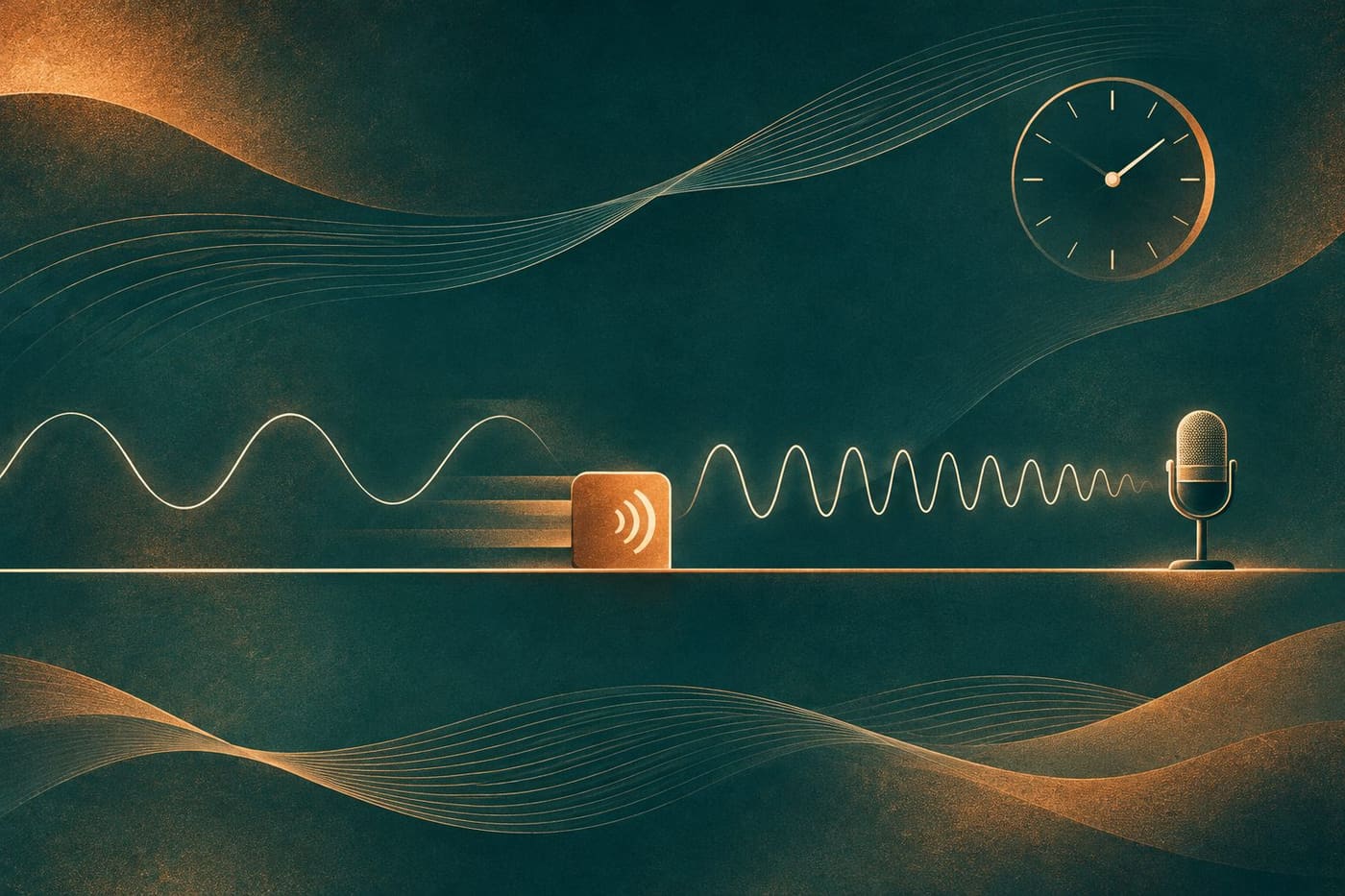
A sound can become louder as its source approaches and also change in pitch. Those are two different observations. Turning a volume control down does not, by itself, explain why a steady passing tone can sound lower after the source has moved away. The Doppler effect concerns the frequency received by an observer when the source, the observer or both move.
This explanation begins with a steady tone and a simple still-air model. It then works through invented numbers to show what the model predicts and where its assumptions matter. The calculations are not recordings of a real vehicle or measurements of anyone's hearing. A passing siren is a familiar starting idea, but understanding the effect does not require treating every change in a real siren as a pure Doppler shift.
Identify the source and the observer
The source is the object producing the sound; the observer is where the sound is received. A microphone can be the observer in an experiment. Before explaining a pitch change, specify which is moving and what the motion is measured relative to. In the first model here, the air and observer are stationary while a source moves at a steady speed below the speed of sound.
NASA Glenn's Doppler explanation describes a moving source emitting sound that propagates through the air. Its key distinction is between the source's motion and the propagation of the disturbances already emitted. The source continues to make the tone while successive parts of the sound leave from different positions.
Draw those roles in a small research sketch before adding any numbers: a source, a receiving position and a direction of travel. Label the assumed air conditions. If a later calculation moves the observer instead, redraw the situation. An identical number beside a different arrow is not necessarily the same physical experiment, even when both examples involve an approaching sound.
Think about successive emissions
The UNSW Physics explanation describes wavefronts spreading from the places where they were emitted. In front of a moving subsonic source, their spacing is smaller; behind it, their spacing is larger. The picture is about a sequence of emissions, not a source dragging every previously emitted wave along with it.
Imagine marking where the source was at each successive emission. The oldest disturbance has had longer to travel than the newest one. If the source advances between emissions, the starting points also advance. Following those separate starting points is more informative than drawing all the expanding wavefronts around the source's latest position.
For a stationary receiver in still air, closer wavefront spacing means more cycles arrive each second, while wider spacing means fewer. That supplies the qualitative prediction before a calculation: the approaching steady source is heard at a higher frequency than its emitted frequency, and the receding source at a lower one. The source need not change its own tone to produce that contrast.
Keep frequency, period and wave speed separate
Frequency counts cycles per second and is measured in hertz. Period is the time for one cycle. Wavelength is a spatial separation, not a duration. For the stationary receiving position in this simple model, multiplying frequency by wavelength gives the wave speed in the medium. Confusing any two of these quantities can create a plausible sentence with the wrong physical meaning.
NASA's speed-of-sound guide relates the propagation speed to properties of the gas. The sound does not gain the source's travel speed simply because the source is approaching. In our model the air conditions are fixed, so the wave speed used in the calculation stays fixed while the spacing and received frequency differ on the two sides.
When checking an explanation, ask what its word faster describes. Does it mean a source travelling faster, a wave propagating faster or more cycles arriving per second? These are separate statements. A useful explanation names the quantity instead of letting one everyday word do three different jobs.
Work through an invented moving-source calculation
Assume a steady emitted frequency of 600 Hz, a sound speed of 340 metres per second and source motion directly toward a stationary receiver at 20 metres per second. These are chosen calculation inputs, not an observed siren, a measured weather condition or a recommended experimental setup. We also assume still, uniform air and no reflected sound.
For this approaching moving-source case, the received frequency equals the emitted frequency multiplied by sound speed divided by sound speed minus source speed. The expression is 600 × 340 / (340 − 20), giving 637.5 Hz. The result is above 600 Hz, as the qualitative reasoning predicted. Both speeds use the same units.
For direct recession at the same speed under the same assumptions, change the denominator to sound speed plus source speed: 600 × 340 / (340 + 20). That gives approximately 566.7 Hz. The OpenStax discussion of the sound Doppler effect explains the moving-source and moving-observer cases separately. The numbers here are our own worked example, not its textbook exercise or experimental results.
Check the arithmetic against the situation
Start with the signs, not with a remembered fraction. In the approaching calculation, the denominator is 320 and the ratio 340/320 is greater than one. In the receding calculation, the denominator is 360 and the ratio 340/360 is less than one. If your approach answer comes out lower than the emitted frequency, revisit which situation and sign you used.
There is another useful check: set the source speed to zero while leaving everything else the same. Both expressions then return 600 Hz. That is the expected stationary result in this model. If a rearrangement fails this check, look for a missing factor or an incorrectly entered denominator before interpreting the answer.
Retain enough digits to compare the calculations, but do not turn rounding into a claim of measurement accuracy. Writing 566.7 Hz means a rounded model result. It does not establish that a real microphone, source or air temperature was known to that precision. Keeping calculation inputs and actual observations in separate columns prevents that confusion.
Cross-check the results with wavelength
The moving-source results can also be checked through wavelength. With the source stationary in the assumed air, 340 divided by 600 gives about 0.567 metres between corresponding wavefronts. With the source moving directly forward at 20 metres per second, the forward spacing in the same model becomes (340 − 20) / 600, about 0.533 metres. Behind the source it becomes (340 + 20) / 600, or 0.600 metres. These are computed spacings, not measurements taken from the conceptual illustration accompanying this article.
At the stationary receiver ahead, dividing the fixed wave speed by that smaller spacing gives 637.5 cycles per second. Behind, dividing by the larger spacing gives approximately 566.7. This is a second way of connecting the same inputs, not independent experimental confirmation. It helps locate a calculation error if a written explanation says the waves are closer together while its numerical wavelength has grown. The assumptions must remain the same during the cross-check; changing the air speed or the observer's motion midway would answer another question.
Moving the observer is a different calculation
Now keep the source stationary and move the observer directly toward it at 20 metres per second through still air. Retain the same assumed 600 Hz tone and 340 metres-per-second wave speed. The wave pattern produced in the air differs from the moving-source case; the observer encounters it at a different rate.
For approach in this second case, use 600 × (340 + 20) / 340, which gives approximately 635.3 Hz. For motion directly away, use 600 × (340 − 20) / 340, approximately 564.7 Hz. Both directions agree with the expected increase or decrease, but the answers are not identical to 637.5 and 566.7 Hz from moving the source.
This contrast is useful because it catches a tempting shortcut: treating every equal closing speed as the same sound problem. The air supplies a medium against which these motions are specified. Keep the source speed, observer speed and sound speed separately labelled. The numerical examples compare two stated models; they are not a method for finding an unknown road speed by ear.
A pass beside you need not make an instantaneous jump
The worked calculations concern direct approach and direct recession. A source passing to one side has changing geometry. UNSW's teaching account explains why an offset passage can produce a smooth transition as the component of motion along the source-observer direction changes. A simplified drawing with two constant values should not be mistaken for the full time history of every real pass.
If you are reading a demonstration, look for a stated path and microphone position. A scene filmed from a distance and a diagram placing a receiver on the source's line are not the same arrangement. Keep the geometry attached to any expected curve rather than judging a recording against an unexplained sketch.
This guide does not calculate the complete changing-path problem. That would require more information about positions, timing and propagation. The modest conclusion is enough for the present purpose: the contrast between approach and recession is meaningful, while the exact shape and timing of a transition depend on the situation being analysed.
A louder tone is not necessarily a higher-frequency tone
OpenStax's sound-intensity section distinguishes the energy carried through an area from the timing of wave cycles. In an ideal outward-spreading wave without energy loss, the same power spreads over a larger area with distance. This helps explain why a sound's level can change without using frequency as the explanation for that change.
For an imagined pair of audio samples, one could have the same cycle rate but a smaller amplitude. Another could have a different cycle rate. Describe the observation you are comparing: level, repetition timing or both. The word lower is ambiguous unless the sentence says lower in pitch or lower in level.
A waveform image also needs labelled axes and context. More closely spaced repetitions along a time axis tell a different story from a taller trace. Do not infer a frequency change merely because someone amplified a quiet part of a demonstration for display. This is a suggestion for reading evidence, not a claim that an audio analysis was performed for this article.
Distinguish a sound analogy from spacecraft radio
NASA JPL's Doppler teaching resource connects a sound demonstration with spacecraft tracking. It describes comparing transmitted and received radio frequencies as part of tracking motion. The connection concerns frequency shifts; it does not mean that spacecraft communication is sound travelling through interplanetary air.
Sound and light cannot simply share the same equation with a different number substituted for the wave speed. The OpenStax explanation for light highlights the difference: light in vacuum needs no material medium, and its Doppler treatment is relativistic. Our 600 Hz still-air calculation is not a spacecraft navigation model.
This boundary makes the analogy more useful. It lets a reader recognise the shared question of emitted and received frequency while retaining the physics that changes between the examples. A familiar demonstration can introduce a concept without carrying every assumption into a different setting.
Read a demonstration with its assumptions attached
Before accepting a numerical result, identify whether the tone was steady, which object moved, what medium was assumed and whether the geometry matched the equation. Keep the source frequency separate from the received value. If the source itself changes tone, a comparison needs to account for that rather than attributing every audible change to motion.
For a learning exercise, a published teaching demonstration or an on-screen model can illustrate the distinction without arranging a roadside experiment. Record what is supplied by the demonstration and what is inferred from a model. Missing source frequency or unclear geometry should remain missing information, not an invitation to invent a precise speed.
More explanations are available in our Science section. The central idea is simple but specific: motion can change how often wave cycles reach an observer, while loudness and propagation speed are different quantities. Sources consulted 6 November 2026: selected NASA, UNSW and OpenStax educational explanations. All numerical inputs and results are worked-model examples, not measurements, hearing tests, traffic estimates or a new experiment.