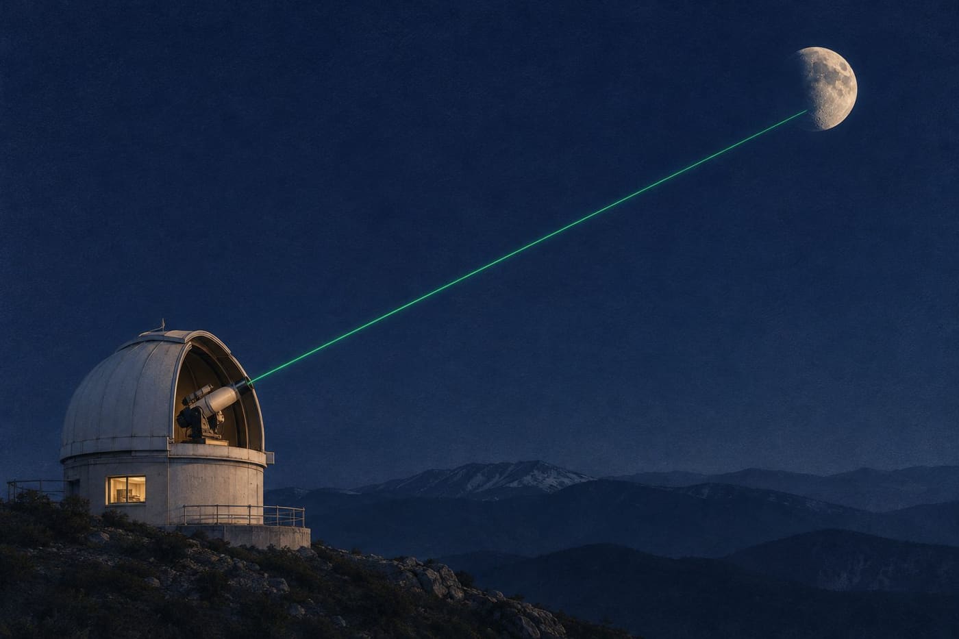
A telescope aimed at the Moon can do more than collect light that was already on its way to Earth. At a lunar laser ranging station, a laser sends a brief pulse towards a reflector on the lunar surface. The telescope then looks for a faint return. A clock records how long the light took to travel out and back. The longer the path, the longer the delay. A measurement that begins with a time interval can help scientists follow the changing geometry of the Earth–Moon system.
The idea sounds like measuring the width of a valley from the delay of an echo. The hard part is recognising the echo and knowing exactly what path it represents. The Moon moves during the measurement, the observing station is carried by Earth’s rotation, and the reflector sits on the lunar surface. The timing is an observation of that particular geometry. To say what it tells us about the whole orbit, scientists have to connect it to many other observations and a model.
Turn a round-trip time into a first estimate
Start with an imaginary pulse that returns after 2.56 seconds. Light travels at approximately 299,792 kilometres per second in vacuum. Multiplying the two gives roughly 767,468 kilometres for the total path. Half is about 383,734 kilometres. The division by two matters because the stopwatch kept running on both legs of the journey. Reporting the full path as the one-way distance would place the target roughly twice as far away.
The example is a first estimate with deliberately rounded inputs. It assumes the two legs can be treated as equal and uses the vacuum speed of light for the entire journey. A real reduction considers the motion of the transmitter, receiver and reflector, and the portion of the path through the atmosphere. The simple calculation remains useful because it gives the scale and shows how an error in timing becomes an error in range. It does not supply the final corrections.
Think about what a rounded time can support. If someone writes down only 2.56 seconds, the missing digits could correspond to a substantial distance. A hundredth of a second in round-trip time represents nearly 1,500 kilometres in the simple one-way calculation. A nanosecond, which is a billionth of a second, represents about 15 centimetres. Those are conversions between units. They do not tell you that a clock with a nanosecond display, or a single photon measured with that clock, automatically delivers a 15-centimetre result.
Two people can also use the word distance to mean different things. One might ask how far a particular telescope is from a reflector. Another might ask how far the centre of Earth is from the centre of the Moon. The telescope is on Earth’s surface and the reflector is on the Moon’s surface. Their separation is a measurement tied to locations and time. The centre-to-centre distance is a quantity that can be calculated from a model that accounts for the offsets and the changing orientations.
Give a faint pulse a way back
The NASA CDDIS lunar laser ranging dataset description explains the basic arrangement. A narrow pulse illuminates corner-cube retroreflectors, and a telescope collects the return. The description notes that the return typically consists of only a few photons. Lunar ranging does not require a picture of the reflector in the receiving telescope. It requires the detection and timing of enough photons that can credibly be associated with the outgoing pulses.
A corner cube uses three mutually perpendicular reflecting surfaces. The direction of a ray reverses along each of the three axes as it reflects, so a ray that makes the necessary reflections exits back towards the direction from which it came. The beam leaving the device can be displaced from the incident ray. The useful feature is the return direction. A flat mirror can also send light back to its source, but only when oriented appropriately to the incoming beam. The corner cube can provide the returning direction over a range of angles.
JPL’s account of the Apollo 11 experiment describes a panel with 100 fused-silica corner cubes. The array is passive. It sends no electronic message and needs no power supply to perform the reflection. If an observer associates a return with the outgoing pulse, the time is measured at the station. A clock on the lunar surface is unnecessary for this arrangement.
Aiming still matters. A laser beam is not an infinitely thin line, and the return does not all enter the telescope. Some transmitted light misses the reflector. Of the light directed back, only a fraction reaches the receiver. This is one reason the station cannot assume each shot will give a clear result. An absence of useful returns during an observation can reflect conditions or pointing as well as the weakness of the signal. It is not, on its own, a measurement of a different lunar distance.
Recognise a return among unrelated detections
If the expected delay is a little over two and a half seconds, a station can predict roughly when a photon should arrive. That prediction comes from the known geometry of the station, the Moon and the reflector. It lets observers concentrate on a time window around the expected return. A photon recorded in that window is a candidate. Other light, and noise in the detector, can also produce detections.
Imagine an illustrative record from repeated pulses. Most shots leave no candidate at all. A few detections appear at unrelated delays. Another group repeatedly falls near the delay predicted for the reflector, after allowing for the way that prediction changes between shots. The group is more informative than one isolated detection. Repetition lets the observer look for a return that follows the expected path and assess how widely the measurements are spread.
The time window has a purpose beyond rejecting irrelevant data. If it is placed incorrectly, it can miss the return entirely. If it is too wide, more unrelated detections compete with it. A model can help find the signal without dictating the measured answer. The distinction is similar to using a street address to find the correct building before measuring its height. The address narrows the search, while the measurement still needs its own evidence.
Records can be combined into a representative result for a series of shots. A combined result can improve the estimate when individual measurements have scatter. That improvement depends on the data and on how the signals are selected and combined. A systematic timing offset can remain even when many measurements agree with one another. That is why the station has to characterise the timing system and report how the data were processed.
Separate timing offsets from the geometry
The interval between the station’s recorded transmit and receive times contains the light-travel time and any unaccounted delays in the equipment. Electronics and optical paths have their own timing behaviour. Calibration gives the observer a way to estimate instrumental delays. Treating those delays as part of the trip to the Moon would shift the inferred range.
The atmosphere matters for a different reason. The light moves through air near the station on both legs. Using the vacuum speed for those portions without a correction would assign the measured delay to the wrong amount of geometric distance. The size of the effect depends in part on the path through the air. The outgoing and returning pulse spend most of their journey outside the atmosphere, but the short portion near the telescope still matters in a precise measurement.
Location and orientation also change. A station moves as Earth rotates. A reflector’s position relative to the lunar centre depends on where the array was placed and how the Moon is oriented. During the time the pulse travels, the two bodies and the station continue to move. A precise calculation models the outgoing and returning legs rather than assuming the telescope and target were motionless while the clock ran.
Notice how these effects differ. A timing bias shifts the measured interval. An atmospheric delay changes the relationship between time and geometric path. A station’s changing position alters the path itself. Listing all three as an unspecified correction would hide the reason each one has to be treated separately. A strong analysis can identify which correction comes from an instrument calibration, which comes from the environment and which comes from the model of motion.
Read a precision claim at the scale it describes
The Apache Point dataset characterization archived by NASA discusses a long series of lunar laser ranging observations and the performance of its timing measurements. A reported precision for that work should be read with its definition and aggregation. Precision can describe the scatter of a set of measurements, an uncertainty assigned to a combined observation, or another property of the reported analysis. It does not mean that every detected photon fixes the centre-to-centre Earth–Moon distance by itself.
There are two useful questions when you see a number. First, which quantity was measured or estimated? A delay, a station-to-reflector range and a parameter fitted from many ranges are distinct. Second, what does the uncertainty describe? If it describes random scatter, a repeatable instrument offset may be a separate concern. If it describes a result combined over many observations, it is not necessarily a typical error for a single shot.
Here is an ordinary analogy. Suppose a set of readings from a ruler differ by a millimetre, but the end of the ruler starts two millimetres away from its marked zero. Repetition can show that the readings are consistent. It cannot reveal or correct the misplaced zero without another check. In ranging, calibration, comparison across stations and scrutiny of the model provide ways to investigate differences that repetition alone cannot resolve.
The same care applies when comparing a modern dataset with a historical experiment. A better instrument can change what the observing team can resolve, but a published figure can also change because it describes a different quantity. Compare the measurement and the conditions before attributing every improvement to a particular device.
Learn what many years of returns can show
An individual observation gives a range tied to one place and moment. A collection of observations can follow how those ranges vary as Earth rotates and the Moon travels in its orbit. NASA’s CDDIS description lists the lunar orbit, rotation and tides among the subjects that can be studied with the data. JPL’s historical account also discusses how long-term measurements contribute to understanding the Earth–Moon system. Those investigations draw on the pattern across observations, along with physical models, rather than on the travel time of one pulse.
The long record also helps distinguish a short-term variation from a persistent effect. If you take two observations on different nights, they can differ because the Moon is in a different part of its orbit and because the two measurements have different geometry. Two numbers are insufficient to estimate a long-term trend without accounting for those changes. Measurements spread across time and geometry give an analysis more ways to tell the effects apart.
When reading about a ranging result, find the target, the station and the interval over which the observations were collected. Look for a clear description of how returns were combined and whether the article is discussing measured ranges or a model fitted to them. If a story uses a single familiar number for the distance to the Moon, ask whether it is an approximate reference, a particular geometric distance or an average over time.
The pulse that left the telescope makes a simple journey in outline. It travels to the Moon, some of its light returns, and a clock measures the delay. Following that delay through the calibration and the geometry shows why lunar ranging is more than a multiplication exercise. Each observation contributes a constraint on where the station and the reflector were relative to one another. The long record turns those constraints into a way to study how the Earth and Moon move together.
For another example of what measurements can reveal about a Solar System object, see the analysis of Bennu samples.
Sources consulted 4 November 2026. The timing example and imagined detection record are illustrative.